【導讀】開源MIT Min cheetah機械狗設計第28篇,番外篇第4篇,Gmapping源碼解讀。
上一篇我們詳細聊了下Gmapping建圖的原理,是一種基於RBpf(Rao-Blackwellized)粒子濾波演算法,即將定位和建圖過程分離,先進行定位再進行建圖,定位與建圖相輔相成、互相影響。
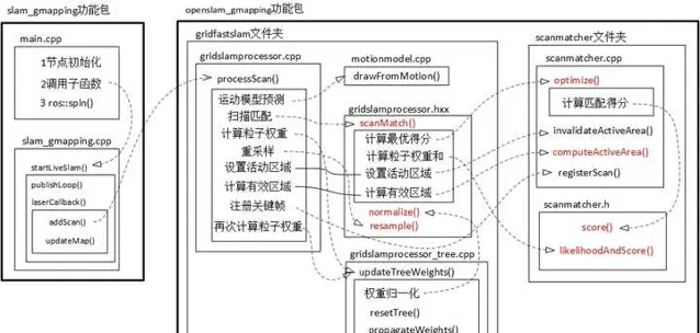
這個作者整理的Gmapping程式碼的框架:Gmapping的個人理解_gmapping框架-CSDN部落格
下面我們會結合程式碼來詳細看看定位和建圖到底是怎麽實作的?
一、問題來源
我們知道,以往的機器人如果要進行定位,必須要先有地圖,反過來,如果想建立地圖,就必須得先知道機器人位置。
顯然上述陷入了先有雞還是先有蛋的問題。
而在Gmapping中,我們將機器人所有時刻位姿 x_{1:t} 和地圖 m 都作為狀態變量,同時對位姿和地圖進行估計,也即:
p(x_{1:t},m|z_{1:t},u_{1:t})---(1)
如果只對當前時刻機器人定位,則公式變為:
p(x_{t}|z_{1:t},u_{1:t},m)
如果對當前時刻機器人定位,同時對地圖進行估計,則公式變為:
p(x_{t},m|z_{1:t},u_{1:t})(註意x下標和上面的區別)
其中: x_{1:t} 為所有歷史機器人位姿, m 為環境地圖, z_{1:t} 為傳感器測試值, u_{1:t} 為輸入控制。
Gmapping的粒子濾波則用的公式(1)
為了求得公式 (1),Gmapping對其進行進一步展開:
透過條件聯合機率分布公式:
p(a,b|c)=p(a|c)p(b|a,c)
對 p(x_{1:t},m|z_{1:t},u_{1:t}) 進行化簡
令 a=x_{1:t} , b=m , c=z_{1:t},u_{1:t} ,則
p(x_{1:t},m|z_{1:t},u_{1:t})=p(x_{1:t}|z_{1:t},u_{1:t})p(m|x_{1:t},z_{1:t},u_{1:t})
又由於 m和u_{1:t}無關 ,因此 p(m|x_{1:t},z_{1:t},u_{1:t})=p(m|x_{1:t},z_{1:t})
即:
p(x_{1:t},m|z_{1:t},u_{1:t})=\frac{p(x_{1:t}|z_{1:t},u_{1:t})}{機器人位姿估計}\frac{p(m|x_{1:t},z_{1:t})}{地圖構建}
其中已知機器人位姿進行地圖構建比較簡單,因此重點就放在機器人位姿估計 \frac{p(x_{1:t}|z_{1:t},u_{1:t})}{機器人位姿估計} 。
但是 \frac{p(x_{1:t}|z_{1:t},u_{1:t})}{機器人位姿估計} 無法直接計算,需要推匯出遞推形式(只有遞推形式才有當前時刻和上一時刻的關聯,才可以實作即時濾波):
即要想辦法找出聯合機率 t 時刻和上一時刻 t-1 時刻的關系:
p(x_{1:t}|z_{1:t},u_{1:t})=\psi *p(x_{1:t-1}|z_{1:t-1},u_{1:t-1})
也即想辦法求出系數 \psi 來建立之間的關系
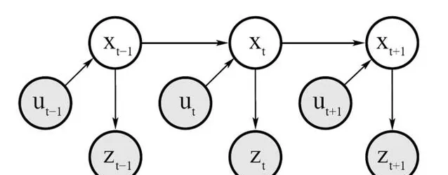
由上面的這個機率圖我們可以看出:
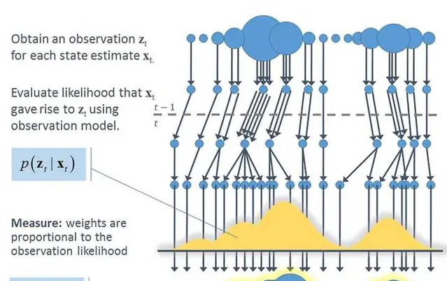
1)測量機率
p(z_{t}|x_{1:t},z_{1:t-1},u_{1:t})=p(z_{t}|x_{t})---(2) 也即 觀測值z_{t} 只與當前時刻的機器人位姿 x_{t} 有關。
2)狀態轉移機率
p(x_{t}|x_{1:t-1},z_{1:t-1},u_{1:t})=p(x_{t}|x_{t-1},u_{t})---(3) 也即當前時刻機器人位姿 x_{t} 只與上一時刻 x_{t-1} 以及控制量 u_{t} 有關。
由(2)和(3)我們可以推導遞迴關係:\frac{p(x_{1:t}|z_{1:t},u_{1:t})}{當前時刻}\\ =p(x_{1:t}|z_{t},u_{1:t},z_{1:t-1})\\ =\eta p(z_{t}|x_{1:t},u_{1:t},z_{1:t-1})p(x_{1:t}|u_{1:t},z_{1:t-1})\\ =\eta p(z_{t}|x_{t})p(x_{1:t}|u_{1:t},z_{1:t-1})\\ =\frac{\eta p(z_{t}|x_{t})p(x_{t}|x_{t-1},u_{t})}{系數}\frac{p(x_{1:t-1}|u_{1:t-1},z_{1:t-1})}{上一時刻}
可以看出機器人軌跡估計就是上一時刻經過運動學機率方程式 p(x_{t}|x_{t-1},u_{t}) 進行傳播,到了當前時刻後,經過觀測機率方程式 p(z_{t}|x_{t}) 進行矯正。
現在的任務就是求這個系數項: p(z_{t}|x_{t})和p(x_{t}|x_{t-1},u_{t})
其中 p(z_{t}|x_{t}) 為觀測機率函式,屬於傳感器探測精度,屬於已知。
主要需要求解 p(x_{t}|x_{t-1},u_{t}) ,這裏就需要使用裏程計運動模型。
二、裏程計運動模型
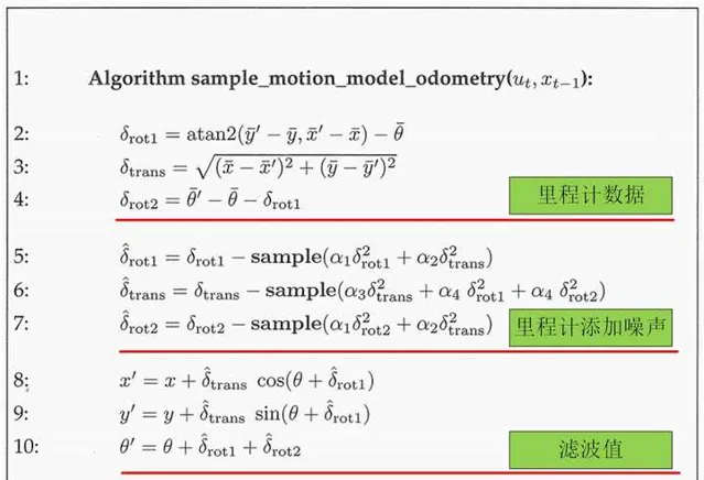
裏程計運動模型主要用來更新下一時刻機器人的位姿,也即 p(x_{t}|u_{t},x_{t-1}) ,即由上一時刻濾波後的值 x_{t-1} 以及裏程計的值 u_{t} 推匯出 x_{t} ,過程如下:
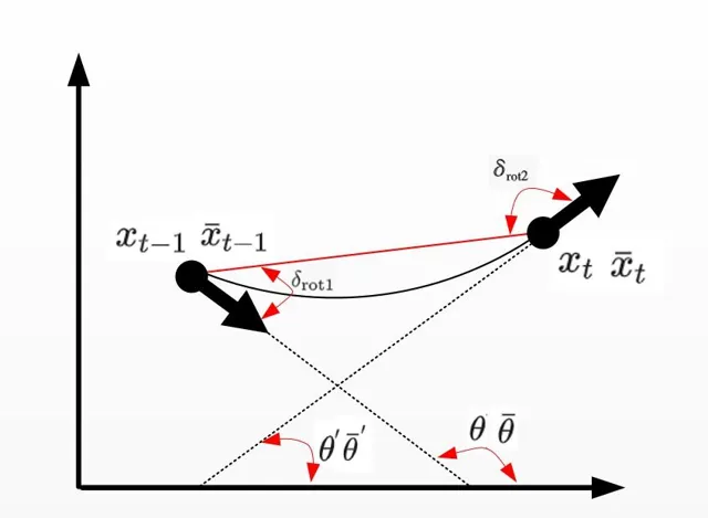
其中 x_{t-1}=[x,y,\theta] ,裏程計讀數 u_{t}=[\bar{x}_{t-1},\bar{x}_{t}] ,其中 \bar{x}_{t-1}=[\bar{x},\bar{y},\bar{\theta}] , \bar{x}_{t}=[\bar{x}^{'},\bar{y}^{'},\bar{\theta}^{'}]
最終機器人姿態 x_{t}=[x^{’},y^{’},\theta^{’}] ,具體演算法如下:
解讀如下:
其中虛擬碼
2-4 : \delta_{rot1} 和 \delta_{rot2} 為機器人內部座標系,即兩個角度是相對的關系,和外界世界座標系沒有關系。
\delta_{trans} 為時刻 t-1和t 機器人的位置連線距離,公式透過上圖簡單的幾何關系可以得到。
5-7 :由於裏程計讀數是有誤差的,因此需要建立運動誤差模型,給真值加上誤差雜訊,假定旋轉和平移的「真」值是用測量值減去均 值為 0、變異數為 b^{2} 的獨立雜訊 \varepsilon_{b^{2}} 。 \varepsilon_{b^{2}} 由sample( \varepsilon_{b^{2}} )函式進行采樣。
其中
\alpha_{1}: 平移運動中平移分量的雜訊
\alpha_{2}: 平移運動中旋轉分量的雜訊
\alpha_{3}: 旋轉運動中平移分量的雜訊
\alpha_{4}: 旋轉運動中旋轉分量的雜訊
\alpha_{1}\sim\alpha_{4} 都屬於機器人地盤固有參數,需要透過實驗獲得。
8-10: 透過幾何關系計算最終濾波後的 x_{t}
程式碼實作:
 MotionModel
 ::
 drawFromMotion
 (
 const
 OrientedPoint
 &
 p
 ,
 const
 OrientedPoint
 &
 pnew
 ,
 const
 OrientedPoint
 &
 pold
 )
 const
 {
 /*
 srr 線性運動造成的線性誤差的變異數
 srt 線性運動造成的角度誤差的變異數
 str 旋轉運動造成的線性誤差的變異數
 stt 旋轉運動造成的角度誤差的變異數
 也即a1-a4
 */
 double
 sxy
 =
 0.3
 *
 srr
 ;
 OrientedPoint
 delta
 =
 absoluteDifference
 (
 pnew
 ,
 pold
 );
 //初始位置相對於結束位置
 OrientedPoint
 noisypoint
 (
 delta
 );
 //初始化一個噪點
 //x,y,theta添加高斯雜訊
 noisypoint
 .
 x
 +=
 sampleGaussian
 (
 srr
 *
 fabs
 (
 delta
 .
 x
 )
 +
 str
 *
 fabs
 (
 delta
 .
 theta
 )
 +
 sxy
 *
 fabs
 (
 delta
 .
 y
 ));
 noisypoint
 .
 y
 +=
 sampleGaussian
 (
 srr
 *
 fabs
 (
 delta
 .
 y
 )
 +
 str
 *
 fabs
 (
 delta
 .
 theta
 )
 +
 sxy
 *
 fabs
 (
 delta
 .
 x
 ));
 noisypoint
 .
 theta
 +=
 sampleGaussian
 (
 stt
 *
 fabs
 (
 delta
 .
 theta
 )
 +
 srt
 *
 sqrt
 (
 delta
 .
 x
 *
 delta
 .
 x
 +
 delta
 .
 y
 *
 delta
 .
 y
 ));
 noisypoint
 .
 theta
 =
 fmod
 (
 noisypoint
 .
 theta
 ,
 2
 *
 M_PI
 );
 if
 (
 noisypoint
 .
 theta
 >
 M_PI
 )
 noisypoint
 .
 theta
 -=
 2
 *
 M_PI
 //將雜訊添加到最優粒子點p上,根據運動模型,得到新的位置
 return
 absoluteSum
 (
 p
 ,
 noisypoint
 );
 }
得到新的位置:
 orientedpoint
 <
 T
 ,
 A
 >
 absoluteSum
 (
 const
 orientedpoint
 <
 T
 ,
 A
 >&
 p1
 ,
 const
 orientedpoint
 <
 T
 ,
 A
 >&
 p2
 ){
 double
 s
 =
 sin
 (
 p1
 .
 theta
 ),
 c
 =
 cos
 (
 p1
 .
 theta
 );
 return
 orientedpoint
 <
 T
 ,
 A
 >
 (
 c
 *
 p2
 .
 x
 -
 s
 *
 p2
 .
 y
 ,
 s
 *
 p2
 .
 x
 +
 c
 *
 p2
 .
 y
 ,
 p2
 .
 theta
 )
 +
 p1
 ;
 }
三、Gmapping建圖座標系
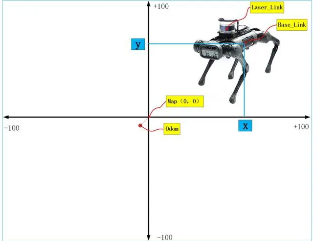
如果建立地圖,首先要搞清除的就是座標系,機器人從開機上電,準備建圖的時,裏程計座標odom和地圖座標map是重合的,但是隨著機器人運動過程中,誤差的累積,odom和map座標系不再重合,也就是說機器人從map出發,裏程計讀數是(10,10),但實際可能就是(9.4,9.4),因此兩座標系是不會重合的。另外Gmapping建立出來的地圖中心在影像的中心,但是像素原點在影像的左下角。而且地圖的尺寸大小可以透過參數進行配置,預設100公尺×100公尺。
四、裏程計數據和雷射雷達數據處理
Gmapping演算法需要的輸入數據:
1、裏程計數據,數據格式為
 header
 :
 timestamp
 :
 2023
 -
 10
 -
 31
 12
 :
 00
 :
 00
 frame_id
 :
 "odom"
 child_frame_id
 :
 "base_link"
 pose
 :
 pose
 :
 position
 :
 //位置資訊
 x
 :
 0.0
 y
 :
 0.0
 z
 :
 0.0
 orientation
 :
 //方位資訊
 x
 :
 0.0
 y
 :
 0.0
 z
 :
 0.0
 w
 :
 0.0
 //共變異數
 covariance
 :
 [
 0.01
 ,
 0
 ,
 0
 ,
 0
 ,
 0
 ,
 0
 ,
 0
 ,
 0.01
 ,
 0
 ,
 0
 ,
 0
 ,
 0
 ,
 0
 ,
 0
 ,
 1000
 ,
 0
 ,
 0
 ,
 0
 ,
 0
 ,
 0.2
 ,
 0
 ,
 0
 ,
 0
 ,
 1000
 ]
 twist
 :
 twist
 :
 linear
 :
 //線速度
 x
 :
 0.0
 y
 :
 0.0
 z
 :
 0.0
 angular
 :
 //角速度
 x
 :
 0.0
 y
 :
 0.0
 z
 :
 0.1
 //共變異數
 covariance
 :
 [
 0.01
 ,
 0
 ,
 0
 ,
 0
 ,
 0
 ,
 0
 ,
 0
 ,
 0.01
 ,
 0
 ,
 0
 ,
 0
 ,
 0
 ,
 0
 ,
 0
 ,
 1000
 ,
 0
 ,
 0
 ,
 0
 ,
 0
 ,
 0.2
 ,
 0
 ,
 0
 ,
 0
 ,
 1000
 ]
2、雷射數據,數據格式為
 Header
 header
 //seq掃描順序增加的ID
 //stamp第一束雷射時間
 //frame_id是掃描的參考系名稱
 int
 seq
 Time
 stamp
 string
 frame_id
 float32
 angle_min
 #
 開始掃描的角度
 (
 角度
 )
 float32
 angle_max
 #
 結束掃描的角度
 (
 角度
 )
 float32
 angle_increment
 #
 每一次掃描增加的角度
 (
 角度
 )
 float32
 time_increment
 #
 測量的時間間隔
 (
 s
 )
 float32
 scan_time
 #
 掃描的時間間隔
 (
 s
 )
 float32
 range_min
 #
 距離最小值
 (
 m
 )
 float32
 range_max
 #
 距離最大值
 (
 m
 )
 float32
 []
 ranges
 #
 距離陣列
 (
 長度
 360
 )(
 註意
 :
 值
 <
 range_min
 或
 >
 range_max
 應當被丟棄
 )
 float32
 []
 intensities
 #
 與裝置有關
 ,
 強度陣列
 (
 長度
 360
 )
其中雷達逆時針0-360,每隔angle_increment儲存一次。最終數據在ranges中。
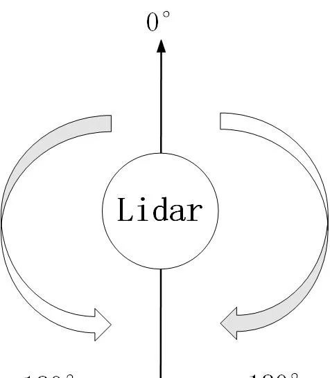
雷射雷達的掃描角度方向:以機器人正前方為0°為基準,順時針為0°-180°,逆時針為0°-負180°
因此需要訂閱這兩個傳感器傳來的數據:
{\color{red}{1、訂閱雷射數據:}}
程式碼:
 scan_filter_sub_
 =
 new
 message_filters
 ::
 Subscriber
 <
 sensor_msgs
 ::
 LaserScan
 >
 (
 node_
 ,
 "scan"
 ,
 5
 );
 scan_filter_
 =
 new
 tf
 ::
 MessageFilter
 <
 sensor_msgs
 ::
 LaserScan
 >
 (
 *
 scan_filter_sub_
 ,
 tf_
 ,
 odom_frame_
 ,
 5
 );
 scan_filter_
 ->
 registerCallback
 (
 boost
 ::
 bind
 (
 &
 SlamGMapping
 ::
 laserCallback
 ,
 this
 ,
 _1
 ));
深拷貝訂閱的雷射雷達測量距離數據ranges_double[]:
 int
 num_ranges
 =
 scan
 .
 ranges
 .
 size
 ();
 for
 (
 int
 i
 =
 0
 ;
 i
 <
 num_ranges
 ;
 i
 ++
 )
 {
 // Must filter out short readings, because the mapper won't
 if
 (
 scan
 .
 ranges
 [
 num_ranges
 -
 i
 -
 1
 ]
 <
 scan
 .
 range_min
 )
 ranges_double
 [
 i
 ]
 =
 (
 double
 )
 scan
 .
 range_max
 ;
 else
 ranges_double
 [
 i
 ]
 =
 (
 double
 )
 scan
 .
 ranges
 [
 num_ranges
 -
 i
 -
 1
 ];
 }
之後將拷貝的雷射雷達數據轉換成Gmapping演算法可以處理的數據形式:
 GMapping
 ::
 RangeReading
 reading
 (
 scan
 .
 ranges
 .
 size
 (),
 ranges_double
 ,
 gsp_laser_
 ,
 scan
 .
 header
 .
 stamp
 .
 toSec
 ());
{\color{red}{2、訂閱裏程計數據:}}
程式實作在getOdomPose()函式中,只是獲得裏程計數據的時候需要和雷射數據關聯起來,單純的獲得雷射數據和裏程計數據是沒有意義的,我們需要獲得的是當前時刻雷射數據對應的當前時刻的裏程計數據,這樣才有意義。
實作的方法就是根據ROS中數據的時間戳來進行關聯。
 //odom_pose為裏程計數據
 tf
 ::
 Stamped
 <
 tf
 ::
 Transform
 >
 odom_pose
 ;
 try
 {
 //得到和雷射數據時間戳對應的裏程計數據
 tf_
 .
 transformPose
 (
 odom_frame_
 ,
 centered_laser_pose_
 ,
 odom_pose
 );
 }
和雷射數據一樣,也需將裏程計數據odom_pose轉化成OrientedPoint數據格式,方便Gmapping演算法計算
 double
 yaw
 =
 tf
 ::
 getYaw
 (
 odom_pose
 .
 getRotation
 ());
 gmap_pose
 =
 GMapping
 ::
 OrientedPoint
 (
 odom_pose
 .
 getOrigin
 ().
 x
 (),
 odom_pose
 .
 getOrigin
 ().
 y
 (),
 yaw
 );
經過上面雷射雷達和裏程計位姿的處理後,就可以為每幀雷射雷達數據設定裏程計位姿
 reading
 .
 setPose
 (
 gmap_pose
 );
可以看出,一個reading裏麵包含了同一時刻雷射的數據和裏程計數據。
五、演算法處理
經過上面數據的獲取後,就可以開始對其進行演算法處理,處理常式為:processScan()
1、取出裏程計位姿數據:
 OrientedPoint
 relPose
 =
 reading
 .
 getPose
 ();
2、 對裏程計位姿數據進行采樣
一個relPose位姿透過運動采樣後變成30個位姿,也即一個粒子變成30個粒子,,得到的新位置再存放在pose中。
 for
 (
 ParticleVector
 ::
 iterator
 it
 =
 m_particles
 .
 begin
 ();
 it
 !=
 m_particles
 .
 end
 ();
 it
 ++
 ){
 OrientedPoint
 &
 pose
 (
 it
 ->
 pose
 );
 pose
 =
 m_motionModel
 .
 drawFromMotion
 (
 it
 ->
 pose
 ,
 relPose
 ,
 m_odoPose
 );
 }
3、更新機器人走的距離和累計的角度
演算法根據機器人走了多少距離或者轉了多少角度來決定要不要呼叫演算法更新地圖,畢竟沒有必要即時的更新地圖,對計算要求挑戰很大。
 OrientedPoint
 move
 =
 relPose
 -
 m_odoPose
 ;
 move
 .
 theta
 =
 atan2
 (
 sin
 (
 move
 .
 theta
 ),
 cos
 (
 move
 .
 theta
 ));
 m_linearDistance
 +=
 sqrt
 (
 move
 *
 move
 );
 m_angularDistance
 +=
 fabs
 (
 move
 .
 theta
 );
 //記錄上一次的裏程計位姿
 m_odoPose
 =
 relPose
 ;
4、取出雷射雷達的測距資訊
 //拷貝拿到雷射雷達的測距數據
 assert
 (
 reading
 .
 size
 ()
 ==
 m_beams
 );
 double
 *
 plainReading
 =
 new
 double
 [
 m_beams
 ];
 for
 (
 unsigned
 int
 i
 =
 0
 ;
 i
 <
 m_beams
 ;
 i
 ++
 ){
 plainReading
 [
 i
 ]
 =
 reading
 [
 i
 ];
 }
 m_infoStream
 <<
 "m_count "
 <<
 m_count
 <<
 endl
 ;
 RangeReading
 *
 reading_copy
 =
 new
 RangeReading
 (
 reading
 .
 size
 (),
 &
 (
 reading
 [
 0
 ]),
 static_cast
 <
 const
 RangeSensor
 *>
 (
 reading
 .
 getSensor
 ()),
 reading
 .
 getTime
 ());
5、在當前位姿下,每個粒子和地圖進行匹配程度打分
函式為scanMatch(),其對每個粒子都進行了匹配得分計算,用到的函式為optimize(),由兩部份組成:
1、對每個粒子進行匹配打分
使用score()函式對每個粒子位姿m_particles[i].pose進行地圖匹配,為每個粒子進行打分,找到最優粒子位姿。
匹配的原理是:透過雷射雷達測距數據和機器人位姿,可以計算出每束雷射在地圖上擊中柵格的位置,這個位置和歷史所有擊中位置的平均值求差值 e ,因此可以用打分公式: Score=e^{\frac{-1}{k*e*e}} 進行打分。 e 越大分越小。
 double
 tmp_score
 =
 exp
 (
 -
 1.0
 /
 m_gaussianSigma
 *
 bestMu
 *
 bestMu
 );
 s
 +=
 tmp_score
 ;
其中參數k,需要調節,使得score的值盡量在0-1之間。
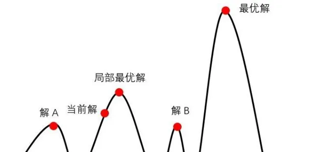
2、透過第1步得到最優位置可能還不是最優的位置,需要在最優位姿附近區域內采樣 n 個位姿進行打分,分為四個方向和兩個轉向進行搜尋,得分比較高的則為最優粒子位姿,使用的是爬山演算法,之所以可以用爬山演算法是因為在最優位姿附近進行小範圍搜尋采樣的樣本認為是符合高斯分布的,高斯分布為單峰函式,因此可以使用爬山演算法。
3、 既然假設n 個位姿采樣符合高斯分布,我們還需要求出期望 \mu 和變異數 \sigma ,這就需要計算每個位姿的權重,並需要進行歸一化,之後加權求和就可以得到期望,進而可以得到變異數,也即最終我們得到的機器人最優位置服從:
x_{t}\sim N(\mu,\sigma^{2})
而權重的計算來自於雷射雷達數據的似然得分:
 m_matcher
 .
 likelihoodAndScore
 (
 s
 ,
 l
 ,
 m_particles
 [
 i
 ].
 map
 ,
 m_particles
 [
 i
 ].
 pose
 ,
 plainReading
 );
權重計算公式:
 double
 f
 =
 (
 -
 1.
 /
 m_likelihoodSigma
 )
 *
 (
 bestMu
 *
 bestMu
 );
 //參數設定m_likelihoodSigma=0.075
累計權重就是粒子權重的累加。
6、 粒子權重歸一化
歸一化函式normalize()函式,其中還有對粒子差異性的判斷,防止粒子耗散:
實作原理是:
假設有 n 個粒子,每個粒子的權重為 w^{i} ,其中權重最大值為 w_{max}
每個粒子經過公式換算後的權重:
w_{變換後}^{i}=e^{\frac{-1}{k*(w^{i}-w_{max})}}
所有粒子變換後的權重進行加和:
w_{所有}+=w_{變換後}^{i}
歸一化:
w_{變換後}^{i}=\frac{w_{變換後}^{i}}{w_{所有}}
得到最終判斷粒子是否發生的耗散的準則:
neff+=w_{變換後}^{i}
neff=\frac{1}{neff}
 //粒子差異化
 m_neff=0;
 for (std::vector<double>::iterator it=m_weights.begin(); it!=m_weights.end(); it++)
 {
 *it=*it/wcum;
 double w=*it;
 m_neff+=w*w;
 }
 m_neff=1./m_neff;
 //粒子權重歸一化
 inline
 void
 GridSlamProcessor
 ::
 normalize
 ()
 {
 */
 /
 normalize
 *
 *
 the
 *
 *
 log
 *
 *
 m_weights
 *
 double
 gain
 =
 1.
 /
 (
 m_obsSigmaGain
 *
 m_particles
 .
 size
 ());
 double
 lmax
 =
 -
 std
 ::
 numeric_limits
 <
 double
 >::
 max
 ();
 for
 (
 ParticleVector
 ::
 iterator
 it
 =
 m_particles
 .
 begin
 ();
 it
 !=
 m_particles
 .
 end
 ();
 it
 ++
 )
 {
 lmax
 =
 it
 ->
 weight
 >
 lmax
 ?
 it
 ->
 weight
 :
 lmax
 ;
 }
 m_weights
 .
 clear
 ();
 double
 wcum
 =
 0
 ;
 m_neff
 =
 0
 ;
 for
 (
 std
 ::
 vector
 <
 Particle
 >::
 iterator
 it
 =
 m_particles
 .
 begin
 ();
 it
 !=
 m_particles
 .
 end
 ();
 it
 ++
 )
 {
 m_weights
 .
 push_back
 (
 exp
 (
 gain
 *
 (
 it
 ->
 weight
 -
 lmax
 )));
 wcum
 +=
 m_weights
 .
 back
 ();
 }
 //粒子差異化
 m_neff
 =
 0
 ;
 for
 (
 std
 ::
 vector
 <
 double
 >::
 iterator
 it
 =
 m_weights
 .
 begin
 ();
 it
 !=
 m_weights
 .
 end
 ();
 it
 ++
 )
 {
 *
 it
 =*
 it
 /
 wcum
 ;
 double
 w
 =*
 it
 ;
 m_neff
 +=
 w
 *
 w
 ;
 }
 m_neff
 =
 1.
 /
 m_neff
 ;
 }
主要程式碼實作:
 inline
 void
 GridSlamProcessor
 ::
 scanMatch
 (
 const
 double
 *
 plainReading
 ){
 double
 sumScore
 =
 0
 ;
 for
 (
 ParticleVector
 ::
 iterator
 it
 =
 m_particles
 .
 begin
 ();
 it
 !=
 m_particles
 .
 end
 ();
 it
 ++
 ){
 OrientedPoint
 corrected
 ;
 double
 score
 ,
 l
 ,
 s
 ;
 //第1步:得到最優匹配位置
 score
 =
 m_matcher
 .
 optimize
 (
 corrected
 ,
 it
 ->
 map
 ,
 it
 ->
 pose
 ,
 plainReading
 );
 if
 (
 score
 >
 m_minimumScore
 ){
 it
 ->
 pose
 =
 corrected
 ;
 }
 else
 {
 if
 (
 m_infoStream
 ){
 m_infoStream
 <<
 "Scan Matching Failed, using odometry. Likelihood="
 <<
 l
 <<
 std
 ::
 endl
 ;
 m_infoStream
 <<
 "lp:"
 <<
 m_lastPartPose
 .
 x
 <<
 " "
 <<
 m_lastPartPose
 .
 y
 <<
 " "
 <<
 m_lastPartPose
 .
 theta
 <<
 std
 ::
 endl
 ;
 m_infoStream
 <<
 "op:"
 <<
 m_odoPose
 .
 x
 <<
 " "
 <<
 m_odoPose
 .
 y
 <<
 " "
 <<
 m_odoPose
 .
 theta
 <<
 std
 ::
 endl
 ;
 }
 }
 //第2步:得到似然權重
 m_matcher
 .
 likelihoodAndScore
 (
 s
 ,
 l
 ,
 it
 ->
 map
 ,
 it
 ->
 pose
 ,
 plainReading
 );
 sumScore
 +=
 score
 ;
 it
 ->
 weight
 +=
 l
 ;
 it
 ->
 weightSum
 +=
 l
 ;
 m_matcher
 .
 invalidateActiveArea
 ();
 m_matcher
 .
 computeActiveArea
 (
 it
 ->
 map
 ,
 it
 ->
 pose
 ,
 plainReading
 );
 }
 double
 ScanMatcher
 ::
 optimize
 (
 OrientedPoint
 &
 pnew
 ,
 const
 ScanMatcherMap
 &
 map
 ,
 const
 OrientedPoint
 &
 init
 ,
 const
 double
 *
 readings
 )
 const
 {
 double
 bestScore
 =-
 1
 ;
 OrientedPoint
 currentPose
 =
 init
 ;
 double
 currentScore
 =
 score
 (
 map
 ,
 currentPose
 ,
 readings
 );
 double
 adelta
 =
 m_optAngularDelta
 ,
 ldelta
 =
 m_optLinearDelta
 ;
 unsigned
 int
 refinement
 =
 0
 ;
 enum
 Move
 {
 Front
 ,
 Back
 ,
 Left
 ,
 Right
 ,
 TurnLeft
 ,
 TurnRight
 ,
 Done
 };
 int
 c_iterations
 =
 0
 ;
 do
 {
 if
 (
 bestScore
 >=
 currentScore
 ){
 refinement
 ++
 ;
 adelta
 *=
 .5
 ;
 ldelta
 *=
 .5
 ;
 }
 bestScore
 =
 currentScore
 ;
 //		cout <<"score="<< currentScore << " refinement=" << refinement;
 //		cout << "pose=" << currentPose.x << " " << currentPose.y << " " << currentPose.theta << endl;
 OrientedPoint
 bestLocalPose
 =
 currentPose
 ;
 OrientedPoint
 localPose
 =
 currentPose
 ;
 Move
 move
 =
 Front
 ;
 do
 {
 localPose
 =
 currentPose
 ;
 switch
 (
 move
 ){
 case
 Front
 :
 localPose
 .
 x
 +=
 ldelta
 ;
 move
 =
 Back
 ;
 break
 ;
 case
 Back
 :
 localPose
 .
 x
 -=
 ldelta
 ;
 move
 =
 Left
 ;
 break
 ;
 case
 Left
 :
 localPose
 .
 y
 -=
 ldelta
 ;
 move
 =
 Right
 ;
 break
 ;
 case
 Right
 :
 localPose
 .
 y
 +=
 ldelta
 ;
 move
 =
 TurnLeft
 ;
 break
 ;
 case
 TurnLeft
 :
 localPose
 .
 theta
 +=
 adelta
 ;
 move
 =
 TurnRight
 ;
 break
 ;
 case
 TurnRight
 :
 localPose
 .
 theta
 -=
 adelta
 ;
 move
 =
 Done
 ;
 break
 ;
 default
 :
 ;
 }
 double
 localScore
 =
 score
 (
 map
 ,
 localPose
 ,
 readings
 );
 if
 (
 localScore
 >
 currentScore
 ){
 currentScore
 =
 localScore
 ;
 bestLocalPose
 =
 localPose
 ;
 }
 c_iterations
 ++
 ;
 }
 while
 (
 move
 !=
 Done
 );
 currentPose
 =
 bestLocalPose
 ;
 //cout << __func__ << "currentScore=" << currentScore<< endl;
 //here we look for the best move;
 }
 while
 (
 currentScore
 >
 bestScore
 ||
 refinement
 <
 m_optRecursiveIterations
 );
 //cout << __func__ << "bestScore=" << bestScore<< endl;
 //cout << __func__ << "iterations=" << c_iterations<< endl;
 pnew
 =
 currentPose
 ;
 return
 bestScore
 ;
 }
7、 粒子重采樣,增加多樣性,增加機器人位姿預測範圍
重采樣函式resample()
重采樣演算法采用轉盤賭演算法,當然這個演算法是有一些缺陷的,感興趣的可以檢視更多的重采樣方法。
演算法實作的基本思想:
比如有15個粒子,經過叠代後,發現有5個粒子權重已經很低了,也就是已經退化了,因此我們需要將其剔除,從剩下的10個中再抽樣5個,保持整體15個粒子不變。
首先求得這10個粒子權重的均值:
interval=\frac{1}{n}\sum_{1}^{10}{w_{t}^{i}}(i=1,2,...10)
隨機抽樣一個初始值:
target=interval*rand(Numer)比如target=interval*10
接著按照如下虛擬碼進行采樣:
for\ \ m=1\ to\ \ 10\ \ do\\target=interval*rand(Numer)\\i=1\\while\ \ target>interval\\i=i+1\\interval+=interval\\end\ \ while\\add \ \ \ x^{i}\\end for\\ 程式碼實作:
 std
 ::
 vector
 <
 Particle
 >
 uniform_resampler
 <
 Particle
 ,
 Numeric
 >::
 resample
 (
 const
 typename
 std
 ::
 vector
 <
 Particle
 >&
 particles
 ,
 int
 nparticles
 )
 const
 {
 Numeric
 cweight
 =
 0
 ;
 //compute the cumulative weights
 unsigned
 int
 n
 =
 0
 ;
 for
 (
 typename
 std
 ::
 vector
 <
 Particle
 >::
 const_iterator
 it
 =
 particles
 .
 begin
 ();
 it
 !=
 particles
 .
 end
 ();
 ++
 it
 ){
 cweight
 +=
 (
 Numeric
 )
 *
 it
 ;
 n
 ++
 ;
 }
 if
 (
 nparticles
 >
 0
 )
 n
 =
 nparticles
 ;
 //weight of the particles after resampling
 double
 uw
 =
 1.
 /
 n
 ;
 //compute the interval
 Numeric
 interval
 =
 cweight
 /
 n
 ;
 //compute the initial target weight
 Numeric
 target
 =
 interval
 *::
 drand48
 ();
 //compute the resampled indexes
 cweight
 =
 0
 ;
 std
 ::
 vector
 <
 Particle
 >
 resampled
 ;
 n
 =
 0
 ;
 unsigned
 int
 i
 =
 0
 ;
 for
 (
 typename
 std
 ::
 vector
 <
 Particle
 >::
 const_iterator
 it
 =
 particles
 .
 begin
 ();
 it
 !=
 particles
 .
 end
 ();
 ++
 it
 ,
 ++
 i
 ){
 cweight
 +=
 (
 Numeric
 )
 *
 it
 ;
 while
 (
 cweight
 >
 target
 ){
 resampled
 .
 push_back
 (
 *
 it
 );
 resampled
 .
 back
 ().
 setWeight
 (
 uw
 );
 target
 +=
 interval
 ;
 }
 }
 return
 resampled
 ;
 }
8、粒子數據結構形式
整個程式碼中粒子的數據結構可謂是最重要的。
節點,由於每個粒子都儲存著歷史的軌跡和地圖,因此需要一個樹結構來儲存這些數據,樹結構是以節點node的形式組織起來的,一個節點包括父節點和子節點,這樣整個節點就可以彼此找到。
 TNode
 (
 const
 OrientedPoint
 &
 pose
 ,
 double
 weight
 ,
 TNode
 *
 parent
 =
 0
 ,
 unsigned
 int
 childs
 =
 0
 );
 /**Destroys a tree node, and consistently updates the tree. If a node whose parent has only one child is deleted,
 also the parent node is deleted. This because the parent will not be reacheable anymore in the trajectory tree.*/
 ~
 TNode
 ();
 /**The pose of the robot*/
 //機器人位姿
 OrientedPoint
 pose
 ;
 //父節點
 TNode
 *
 parent
 ;
 /**The range reading to which this node is associated*/
 //雷射雷達數據
 const
 RangeReading
 *
 reading
 ;
 };
粒子數據結構:
 struct
 Particle
 {
 Particle
 (
 const
 ScanMatcherMap
 &
 map
 );
 /** @returns the weight of a particle */
 inline
 operator
 double
 ()
 const
 {
 return
 weight
 ;}
 /** @returns the pose of a particle */
 inline
 operator
 OrientedPoint
 ()
 const
 {
 return
 pose
 ;}
 /** sets the weight of a particle
 @param w the weight
 */
 inline
 void
 setWeight
 (
 double
 w
 )
 {
 weight
 =
 w
 ;}
 /** The map */
 ScanMatcherMap
 map
 ;
 /** The pose of the robot */
 OrientedPoint
 pose
 ;
 /** The pose of the robot at the previous time frame (used for computing thr odometry displacements) */
 OrientedPoint
 previousPose
 ;
 /** The weight of the particle */
 double
 weight
 ;
 /** The cumulative weight of the particle */
 double
 weightSum
 ;
 double
 gweight
 ;
 /** The index of the previous particle in the trajectory tree */
 int
 previousIndex
 ;
 /** Entry to the trajectory tree */
 TNode
 *
 node
 ;
 };
六、地圖更新
用到的函式為:updateMap()
知乎作者的一篇文章,說明了占據地圖是如何建立的,這裏就不再介紹了。
小白學移動機器人:占據柵格地圖構建(Occupancy Grid Map)
 SlamGMapping
 ::
 updateMap
 (
 const
 sensor_msgs
 ::
 LaserScan
 &
 scan
 )
 {
 ROS_DEBUG
 (
 "Update map"
 );
 boost
 ::
 mutex
 ::
 scoped_lock
 map_lock
 (
 map_mutex_
 );
 GMapping
 ::
 ScanMatcher
 matcher
 ;
 matcher
 .
 setLaserParameters
 (
 scan
 .
 ranges
 .
 size
 (),
 &
 (
 laser_angles_
 [
 0
 ]),
 gsp_laser_
 ->
 getPose
 ());
 matcher
 .
 setlaserMaxRange
 (
 maxRange_
 );
 matcher
 .
 setusableRange
 (
 maxUrange_
 );
 matcher
 .
 setgenerateMap
 (
 true
 );
 GMapping
 ::
 GridSlamProcessor
 ::
 Particle
 best
 =
 gsp_
 ->
 getParticles
 ()[
 gsp_
 ->
 getBestParticleIndex
 ()];
 std_msgs
 ::
 Float64
 entropy
 ;
 entropy
 .
 data
 =
 computePoseEntropy
 ();
 if
 (
 entropy
 .
 data
 >
 0.0
 )
 entropy_publisher_
 .
 publish
 (
 entropy
 );
 if
 (
 !
 got_map_
 )
 {
 map_
 .
 map
 .
 info
 .
 resolution
 =
 delta_
 ;
 map_
 .
 map
 .
 info
 .
 origin
 .
 position
 .
 x
 =
 0.0
 ;
 map_
 .
 map
 .
 info
 .
 origin
 .
 position
 .
 y
 =
 0.0
 ;
 map_
 .
 map
 .
 info
 .
 origin
 .
 position
 .
 z
 =
 0.0
 ;
 map_
 .
 map
 .
 info
 .
 origin
 .
 orientation
 .
 x
 =
 0.0
 ;
 map_
 .
 map
 .
 info
 .
 origin
 .
 orientation
 .
 y
 =
 0.0
 ;
 map_
 .
 map
 .
 info
 .
 origin
 .
 orientation
 .
 z
 =
 0.0
 ;
 map_
 .
 map
 .
 info
 .
 origin
 .
 orientation
 .
 w
 =
 1.0
 ;
 }
 GMapping
 ::
 Point
 center
 ;
 center
 .
 x
 =
 (
 xmin_
 +
 xmax_
 )
 /
 2.0
 ;
 center
 .
 y
 =
 (
 ymin_
 +
 ymax_
 )
 /
 2.0
 ;
 GMapping
 ::
 ScanMatcherMap
 smap
 (
 center
 ,
 xmin_
 ,
 ymin_
 ,
 xmax_
 ,
 ymax_
 ,
 delta_
 );
 ROS_DEBUG
 (
 "Trajectory tree:"
 );
 for
 (
 GMapping
 ::
 GridSlamProcessor
 ::
 TNode
 *
 n
 =
 best
 .
 node
 ;
 n
 ;
 n
 =
 n
 ->
 parent
 )
 {
 ROS_DEBUG
 (
 " %.3f %.3f %.3f"
 ,
 n
 ->
 pose
 .
 x
 ,
 n
 ->
 pose
 .
 y
 ,
 n
 ->
 pose
 .
 theta
 );
 if
 (
 !
 n
 ->
 reading
 )
 {
 ROS_DEBUG
 (
 "Reading is NULL"
 );
 continue
 ;
 }
 matcher
 .
 invalidateActiveArea
 ();
 matcher
 .
 computeActiveArea
 (
 smap
 ,
 n
 ->
 pose
 ,
 &
 ((
 *
 n
 ->
 reading
 )[
 0
 ]));
 matcher
 .
 registerScan
 (
 smap
 ,
 n
 ->
 pose
 ,
 &
 ((
 *
 n
 ->
 reading
 )[
 0
 ]));
 }
 // the map may have expanded, so resize ros message as well
 if
 (
 map_
 .
 map
 .
 info
 .
 width
 !=
 (
 unsigned
 int
 )
 smap
 .
 getMapSizeX
 ()
 ||
 map_
 .
 map
 .
 info
 .
 height
 !=
 (
 unsigned
 int
 )
 smap
 .
 getMapSizeY
 ())
 {
 // NOTE: The results of ScanMatcherMap::getSize() are different from the parameters given to the constructor
 // so we must obtain the bounding box in a different way
 GMapping
 ::
 Point
 wmin
 =
 smap
 .
 map2world
 (
 GMapping
 ::
 IntPoint
 (
 0
 ,
 0
 ));
 GMapping
 ::
 Point
 wmax
 =
 smap
 .
 map2world
 (
 GMapping
 ::
 IntPoint
 (
 smap
 .
 getMapSizeX
 (),
 smap
 .
 getMapSizeY
 ()));
 xmin_
 =
 wmin
 .
 x
 ;
 ymin_
 =
 wmin
 .
 y
 ;
 xmax_
 =
 wmax
 .
 x
 ;
 ymax_
 =
 wmax
 .
 y
 ;
 ROS_DEBUG
 (
 "map size is now %dx%d pixels (%f,%f)-(%f, %f)"
 ,
 smap
 .
 getMapSizeX
 (),
 smap
 .
 getMapSizeY
 (),
 xmin_
 ,
 ymin_
 ,
 xmax_
 ,
 ymax_
 );
 map_
 .
 map
 .
 info
 .
 width
 =
 smap
 .
 getMapSizeX
 ();
 map_
 .
 map
 .
 info
 .
 height
 =
 smap
 .
 getMapSizeY
 ();
 map_
 .
 map
 .
 info
 .
 origin
 .
 position
 .
 x
 =
 xmin_
 ;
 map_
 .
 map
 .
 info
 .
 origin
 .
 position
 .
 y
 =
 ymin_
 ;
 map_
 .
 map
 .
 data
 .
 resize
 (
 map_
 .
 map
 .
 info
 .
 width
 *
 map_
 .
 map
 .
 info
 .
 height
 );
 ROS_DEBUG
 (
 "map origin: (%f, %f)"
 ,
 map_
 .
 map
 .
 info
 .
 origin
 .
 position
 .
 x
 ,
 map_
 .
 map
 .
 info
 .
 origin
 .
 position
 .
 y
 );
 }
 for
 (
 int
 x
 =
 0
 ;
 x
 <
 smap
 .
 getMapSizeX
 ();
 x
 ++
 )
 {
 for
 (
 int
 y
 =
 0
 ;
 y
 <
 smap
 .
 getMapSizeY
 ();
 y
 ++
 )
 {
 /// @todo Sort out the unknown vs. free vs. obstacle thresholding
 GMapping
 ::
 IntPoint
 p
 (
 x
 ,
 y
 );
 double
 occ
 =
 smap
 .
 cell
 (
 p
 );
 assert
 (
 occ
 <=
 1.0
 );
 if
 (
 occ
 <
 0
 )
 map_
 .
 map
 .
 data
 [
 MAP_IDX
 (
 map_
 .
 map
 .
 info
 .
 width
 ,
 x
 ,
 y
 )]
 =
 -
 1
 ;
 else
 if
 (
 occ
 >
 occ_thresh_
 )
 {
 //map_.map.data[MAP_IDX(map_.map.info.width, x, y)] = (int)round(occ*100.0);
 map_
 .
 map
 .
 data
 [
 MAP_IDX
 (
 map_
 .
 map
 .
 info
 .
 width
 ,
 x
 ,
 y
 )]
 =
 100
 ;
 }
 else
 map_
 .
 map
 .
 data
 [
 MAP_IDX
 (
 map_
 .
 map
 .
 info
 .
 width
 ,
 x
 ,
 y
 )]
 =
 0
 ;
 }
 }
 got_map_
 =
 true
 ;
 //make sure to set the header information on the map
 map_
 .
 map
 .
 header
 .
 stamp
 =
 ros
 ::
 Time
 ::
 now
 ();
 map_
 .
 map
 .
 header
 .
 frame_id
 =
 tf_
 .
 resolve
 (
 map_frame_
 );
 sst_
 .
 publish
 (
 map_
 .
 map
 );
 sstm_
 .
 publish
 (
 map_
 .
 map
 .
 info
 );
 }
七、結束語
最後,GMapping不是萬能的,它只是在特定歷史時期提出的當時最好的方案。比如Gmapping參考了裏程計的數據,可以使建圖更精確,相比於Hector SLAM,GMapping對雷射雷達頻率要求低、魯棒性更高。
但一旦裏程計打滑,GMapping地圖建立就會出現問題,一般會結合多傳感器和障礙物點雲匹配來進行矯正。
如今,一提到SLAM建圖,都少不了谷歌的Cartographer,在實用性方面其霸主地位迄今也無法撼動。
但GMapping作為特定時代的產物,依然有許多值得借鑒的東西,程式簡潔的架構和思想,依然非常值得我們學習,註定在SLAM的歷史上留下濃墨重彩的一筆。


