【导读】开源MIT Min cheetah机械狗设计第28篇,番外篇第4篇,Gmapping源码解读。
上一篇我们详细聊了下Gmapping建图的原理,是一种基于RBpf(Rao-Blackwellized)粒子滤波算法,即将定位和建图过程分离,先进行定位再进行建图,定位与建图相辅相成、互相影响。
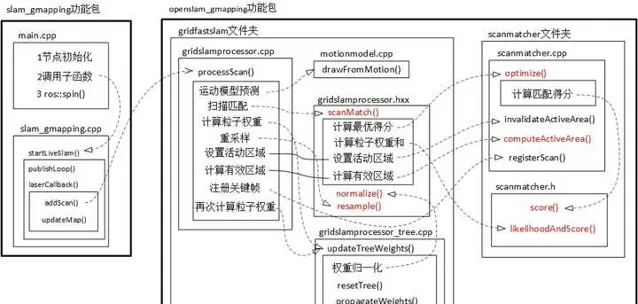
这个作者整理的Gmapping代码的框架:Gmapping的个人理解_gmapping框架-CSDN博客
下面我们会结合代码来详细看看定位和建图到底是怎么实现的?
一、问题来源
我们知道,以往的机器人如果要进行定位,必须要先有地图,反过来,如果想创建地图,就必须得先知道机器人位置。
显然上述陷入了先有鸡还是先有蛋的问题。
而在Gmapping中,我们将机器人所有时刻位姿 x_{1:t} 和地图 m 都作为状态变量,同时对位姿和地图进行估计,也即:
p(x_{1:t},m|z_{1:t},u_{1:t})---(1)
如果只对当前时刻机器人定位,则公式变为:
p(x_{t}|z_{1:t},u_{1:t},m)
如果对当前时刻机器人定位,同时对地图进行估计,则公式变为:
p(x_{t},m|z_{1:t},u_{1:t})(注意x下标和上面的区别)
其中: x_{1:t} 为所有历史机器人位姿, m 为环境地图, z_{1:t} 为传感器测试值, u_{1:t} 为输入控制。
Gmapping的粒子滤波则用的公式(1)
为了求得公式 (1),Gmapping对其进行进一步展开:
通过条件联合概率分布公式:
p(a,b|c)=p(a|c)p(b|a,c)
对 p(x_{1:t},m|z_{1:t},u_{1:t}) 进行化简
令 a=x_{1:t} , b=m , c=z_{1:t},u_{1:t} ,则
p(x_{1:t},m|z_{1:t},u_{1:t})=p(x_{1:t}|z_{1:t},u_{1:t})p(m|x_{1:t},z_{1:t},u_{1:t})
又由于 m和u_{1:t}无关 ,因此 p(m|x_{1:t},z_{1:t},u_{1:t})=p(m|x_{1:t},z_{1:t})
即:
p(x_{1:t},m|z_{1:t},u_{1:t})=\frac{p(x_{1:t}|z_{1:t},u_{1:t})}{机器人位姿估计}\frac{p(m|x_{1:t},z_{1:t})}{地图构建}
其中已知机器人位姿进行地图构建比较简单,因此重点就放在机器人位姿估计 \frac{p(x_{1:t}|z_{1:t},u_{1:t})}{机器人位姿估计} 。
但是 \frac{p(x_{1:t}|z_{1:t},u_{1:t})}{机器人位姿估计} 无法直接计算,需要推导出递推形式(只有递推形式才有当前时刻和上一时刻的关联,才可以实现实时滤波):
即要想办法找出联合概率 t 时刻和上一时刻 t-1 时刻的关系:
p(x_{1:t}|z_{1:t},u_{1:t})=\psi *p(x_{1:t-1}|z_{1:t-1},u_{1:t-1})
也即想办法求出系数 \psi 来建立之间的关系
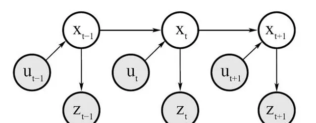
由上面的这个概率图我们可以看出:
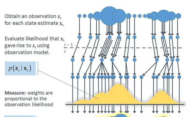
1)测量概率
p(z_{t}|x_{1:t},z_{1:t-1},u_{1:t})=p(z_{t}|x_{t})---(2) 也即 观测值z_{t} 只与当前时刻的机器人位姿 x_{t} 有关。
2)状态转移概率
p(x_{t}|x_{1:t-1},z_{1:t-1},u_{1:t})=p(x_{t}|x_{t-1},u_{t})---(3) 也即当前时刻机器人位姿 x_{t} 只与上一时刻 x_{t-1} 以及控制量 u_{t} 有关。
由(2)和(3)我们可以推导递推关系:\frac{p(x_{1:t}|z_{1:t},u_{1:t})}{当前时刻}\\ =p(x_{1:t}|z_{t},u_{1:t},z_{1:t-1})\\ =\eta p(z_{t}|x_{1:t},u_{1:t},z_{1:t-1})p(x_{1:t}|u_{1:t},z_{1:t-1})\\ =\eta p(z_{t}|x_{t})p(x_{1:t}|u_{1:t},z_{1:t-1})\\ =\frac{\eta p(z_{t}|x_{t})p(x_{t}|x_{t-1},u_{t})}{系数}\frac{p(x_{1:t-1}|u_{1:t-1},z_{1:t-1})}{上一时刻}
可以看出机器人轨迹估计就是上一时刻经过运动学概率方程 p(x_{t}|x_{t-1},u_{t}) 进行传播,到了当前时刻后,经过观测概率方程 p(z_{t}|x_{t}) 进行矫正。
现在的任务就是求这个系数项: p(z_{t}|x_{t})和p(x_{t}|x_{t-1},u_{t})
其中 p(z_{t}|x_{t}) 为观测概率函数,属于传感器探测精度,属于已知。
主要需要求解 p(x_{t}|x_{t-1},u_{t}) ,这里就需要使用里程计运动模型。
二、里程计运动模型
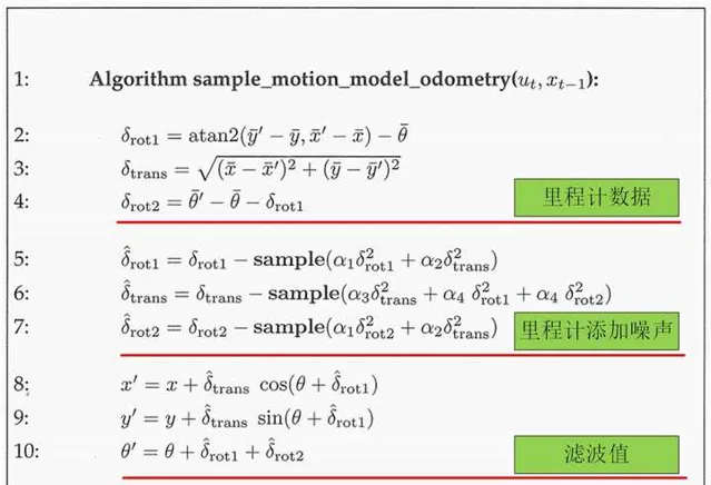
里程计运动模型主要用来更新下一时刻机器人的位姿,也即 p(x_{t}|u_{t},x_{t-1}) ,即由上一时刻滤波后的值 x_{t-1} 以及里程计的值 u_{t} 推导出 x_{t} ,过程如下:
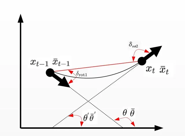
其中 x_{t-1}=[x,y,\theta] ,里程计读数 u_{t}=[\bar{x}_{t-1},\bar{x}_{t}] ,其中 \bar{x}_{t-1}=[\bar{x},\bar{y},\bar{\theta}] , \bar{x}_{t}=[\bar{x}^{'},\bar{y}^{'},\bar{\theta}^{'}]
最终机器人姿态 x_{t}=[x^{’},y^{’},\theta^{’}] ,具体算法如下:
解读如下:
其中伪代码
2-4 : \delta_{rot1} 和 \delta_{rot2} 为机器人内部坐标系,即两个角度是相对的关系,和外界世界坐标系没有关系。
\delta_{trans} 为时刻 t-1和t 机器人的位置连线距离,公式通过上图简单的几何关系可以得到。
5-7 :由于里程计读数是有误差的,因此需要建立运动误差模型,给真值加上误差噪声,假定旋转和平移的「真」值是用测量值减去均 值为 0、方差为 b^{2} 的独立噪声 \varepsilon_{b^{2}} 。 \varepsilon_{b^{2}} 由sample( \varepsilon_{b^{2}} )函数进行采样。
其中
\alpha_{1}: 平移运动中平移分量的噪声
\alpha_{2}: 平移运动中旋转分量的噪声
\alpha_{3}: 旋转运动中平移分量的噪声
\alpha_{4}: 旋转运动中旋转分量的噪声
\alpha_{1}\sim\alpha_{4} 都属于机器人地盘固有参数,需要通过实验获得。
8-10: 通过几何关系计算最终滤波后的 x_{t}
代码实现:
 MotionModel
 ::
 drawFromMotion
 (
 const
 OrientedPoint
 &
 p
 ,
 const
 OrientedPoint
 &
 pnew
 ,
 const
 OrientedPoint
 &
 pold
 )
 const
 {
 /*
 srr 线性运动造成的线性误差的方差
 srt 线性运动造成的角度误差的方差
 str 旋转运动造成的线性误差的方差
 stt 旋转运动造成的角度误差的方差
 也即a1-a4
 */
 double
 sxy
 =
 0.3
 *
 srr
 ;
 OrientedPoint
 delta
 =
 absoluteDifference
 (
 pnew
 ,
 pold
 );
 //初始位置相对于结束位置
 OrientedPoint
 noisypoint
 (
 delta
 );
 //初始化一个噪点
 //x,y,theta添加高斯噪声
 noisypoint
 .
 x
 +=
 sampleGaussian
 (
 srr
 *
 fabs
 (
 delta
 .
 x
 )
 +
 str
 *
 fabs
 (
 delta
 .
 theta
 )
 +
 sxy
 *
 fabs
 (
 delta
 .
 y
 ));
 noisypoint
 .
 y
 +=
 sampleGaussian
 (
 srr
 *
 fabs
 (
 delta
 .
 y
 )
 +
 str
 *
 fabs
 (
 delta
 .
 theta
 )
 +
 sxy
 *
 fabs
 (
 delta
 .
 x
 ));
 noisypoint
 .
 theta
 +=
 sampleGaussian
 (
 stt
 *
 fabs
 (
 delta
 .
 theta
 )
 +
 srt
 *
 sqrt
 (
 delta
 .
 x
 *
 delta
 .
 x
 +
 delta
 .
 y
 *
 delta
 .
 y
 ));
 noisypoint
 .
 theta
 =
 fmod
 (
 noisypoint
 .
 theta
 ,
 2
 *
 M_PI
 );
 if
 (
 noisypoint
 .
 theta
 >
 M_PI
 )
 noisypoint
 .
 theta
 -=
 2
 *
 M_PI
 //将噪声添加到最优粒子点p上,根据运动模型,得到新的位置
 return
 absoluteSum
 (
 p
 ,
 noisypoint
 );
 }
得到新的位置:
 orientedpoint
 <
 T
 ,
 A
 >
 absoluteSum
 (
 const
 orientedpoint
 <
 T
 ,
 A
 >&
 p1
 ,
 const
 orientedpoint
 <
 T
 ,
 A
 >&
 p2
 ){
 double
 s
 =
 sin
 (
 p1
 .
 theta
 ),
 c
 =
 cos
 (
 p1
 .
 theta
 );
 return
 orientedpoint
 <
 T
 ,
 A
 >
 (
 c
 *
 p2
 .
 x
 -
 s
 *
 p2
 .
 y
 ,
 s
 *
 p2
 .
 x
 +
 c
 *
 p2
 .
 y
 ,
 p2
 .
 theta
 )
 +
 p1
 ;
 }
三、Gmapping建图坐标系
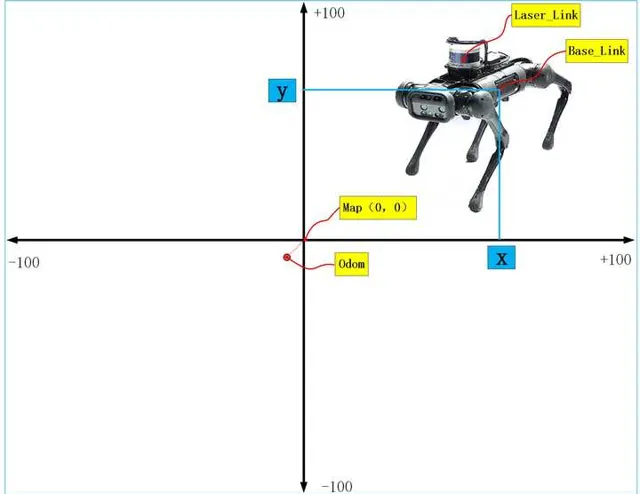
如果建立地图,首先要搞清除的就是坐标系,机器人从开机上电,准备建图的时,里程计坐标odom和地图坐标map是重合的,但是随着机器人运动过程中,误差的累积,odom和map坐标系不再重合,也就是说机器人从map出发,里程计读数是(10,10),但实际可能就是(9.4,9.4),因此两坐标系是不会重合的。另外Gmapping创建出来的地图中心在图像的中心,但是像素原点在图像的左下角。而且地图的尺寸大小可以通过参数进行配置,默认100米×100米。
四、里程计数据和激光雷达数据处理
Gmapping算法需要的输入数据:
1、里程计数据,数据格式为
 header
 :
 timestamp
 :
 2023
 -
 10
 -
 31
 12
 :
 00
 :
 00
 frame_id
 :
 "odom"
 child_frame_id
 :
 "base_link"
 pose
 :
 pose
 :
 position
 :
 //位置信息
 x
 :
 0.0
 y
 :
 0.0
 z
 :
 0.0
 orientation
 :
 //方位信息
 x
 :
 0.0
 y
 :
 0.0
 z
 :
 0.0
 w
 :
 0.0
 //协方差
 covariance
 :
 [
 0.01
 ,
 0
 ,
 0
 ,
 0
 ,
 0
 ,
 0
 ,
 0
 ,
 0.01
 ,
 0
 ,
 0
 ,
 0
 ,
 0
 ,
 0
 ,
 0
 ,
 1000
 ,
 0
 ,
 0
 ,
 0
 ,
 0
 ,
 0.2
 ,
 0
 ,
 0
 ,
 0
 ,
 1000
 ]
 twist
 :
 twist
 :
 linear
 :
 //线速度
 x
 :
 0.0
 y
 :
 0.0
 z
 :
 0.0
 angular
 :
 //角速度
 x
 :
 0.0
 y
 :
 0.0
 z
 :
 0.1
 //协方差
 covariance
 :
 [
 0.01
 ,
 0
 ,
 0
 ,
 0
 ,
 0
 ,
 0
 ,
 0
 ,
 0.01
 ,
 0
 ,
 0
 ,
 0
 ,
 0
 ,
 0
 ,
 0
 ,
 1000
 ,
 0
 ,
 0
 ,
 0
 ,
 0
 ,
 0.2
 ,
 0
 ,
 0
 ,
 0
 ,
 1000
 ]
2、激光数据,数据格式为
 Header
 header
 //seq扫描顺序增加的ID
 //stamp第一束激光时间
 //frame_id是扫描的参考系名称
 int
 seq
 Time
 stamp
 string
 frame_id
 float32
 angle_min
 #
 开始扫描的角度
 (
 角度
 )
 float32
 angle_max
 #
 结束扫描的角度
 (
 角度
 )
 float32
 angle_increment
 #
 每一次扫描增加的角度
 (
 角度
 )
 float32
 time_increment
 #
 测量的时间间隔
 (
 s
 )
 float32
 scan_time
 #
 扫描的时间间隔
 (
 s
 )
 float32
 range_min
 #
 距离最小值
 (
 m
 )
 float32
 range_max
 #
 距离最大值
 (
 m
 )
 float32
 []
 ranges
 #
 距离数组
 (
 长度
 360
 )(
 注意
 :
 值
 <
 range_min
 或
 >
 range_max
 应当被丢弃
 )
 float32
 []
 intensities
 #
 与设备有关
 ,
 强度数组
 (
 长度
 360
 )
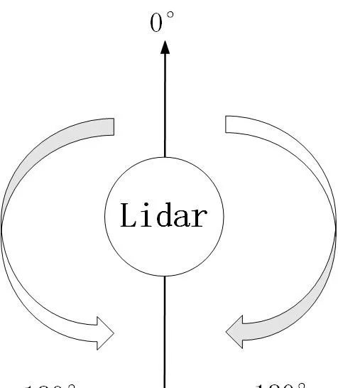
其中雷达逆时针0-360,每隔angle_increment存储一次。最终数据在ranges中。
激光雷达的扫描角度方向:以机器人正前方为0°为基准,顺时针为0°-180°,逆时针为0°-负180°
因此需要订阅这两个传感器传来的数据:
{\color{red}{1、订阅激光数据:}}
代码:
 scan_filter_sub_
 =
 new
 message_filters
 ::
 Subscriber
 <
 sensor_msgs
 ::
 LaserScan
 >
 (
 node_
 ,
 "scan"
 ,
 5
 );
 scan_filter_
 =
 new
 tf
 ::
 MessageFilter
 <
 sensor_msgs
 ::
 LaserScan
 >
 (
 *
 scan_filter_sub_
 ,
 tf_
 ,
 odom_frame_
 ,
 5
 );
 scan_filter_
 ->
 registerCallback
 (
 boost
 ::
 bind
 (
 &
 SlamGMapping
 ::
 laserCallback
 ,
 this
 ,
 _1
 ));
深拷贝订阅的激光雷达测量距离数据ranges_double[]:
 int
 num_ranges
 =
 scan
 .
 ranges
 .
 size
 ();
 for
 (
 int
 i
 =
 0
 ;
 i
 <
 num_ranges
 ;
 i
 ++
 )
 {
 // Must filter out short readings, because the mapper won't
 if
 (
 scan
 .
 ranges
 [
 num_ranges
 -
 i
 -
 1
 ]
 <
 scan
 .
 range_min
 )
 ranges_double
 [
 i
 ]
 =
 (
 double
 )
 scan
 .
 range_max
 ;
 else
 ranges_double
 [
 i
 ]
 =
 (
 double
 )
 scan
 .
 ranges
 [
 num_ranges
 -
 i
 -
 1
 ];
 }
之后将拷贝的激光雷达数据转换成Gmapping算法可以处理的数据形式:
 GMapping
 ::
 RangeReading
 reading
 (
 scan
 .
 ranges
 .
 size
 (),
 ranges_double
 ,
 gsp_laser_
 ,
 scan
 .
 header
 .
 stamp
 .
 toSec
 ());
{\color{red}{2、订阅里程计数据:}}
程序实现在getOdomPose()函数中,只是获得里程计数据的时候需要和激光数据关联起来,单纯的获得激光数据和里程计数据是没有意义的,我们需要获得的是当前时刻激光数据对应的当前时刻的里程计数据,这样才有意义。
实现的方法就是根据ROS中数据的时间戳来进行关联。
 //odom_pose为里程计数据
 tf
 ::
 Stamped
 <
 tf
 ::
 Transform
 >
 odom_pose
 ;
 try
 {
 //得到和激光数据时间戳对应的里程计数据
 tf_
 .
 transformPose
 (
 odom_frame_
 ,
 centered_laser_pose_
 ,
 odom_pose
 );
 }
和激光数据一样,也需将里程计数据odom_pose转化成OrientedPoint数据格式,方便Gmapping算法计算
 double
 yaw
 =
 tf
 ::
 getYaw
 (
 odom_pose
 .
 getRotation
 ());
 gmap_pose
 =
 GMapping
 ::
 OrientedPoint
 (
 odom_pose
 .
 getOrigin
 ().
 x
 (),
 odom_pose
 .
 getOrigin
 ().
 y
 (),
 yaw
 );
经过上面激光雷达和里程计位姿的处理后,就可以为每帧激光雷达数据设置里程计位姿
 reading
 .
 setPose
 (
 gmap_pose
 );
可以看出,一个reading里面包含了同一时刻激光的数据和里程计数据。
五、算法处理
经过上面数据的获取后,就可以开始对其进行算法处理,处理函数为:processScan()
1、取出里程计位姿数据:
 OrientedPoint
 relPose
 =
 reading
 .
 getPose
 ();
2、 对里程计位姿数据进行采样
一个relPose位姿通过运动采样后变成30个位姿,也即一个粒子变成30个粒子,,得到的新位置再存放在pose中。
 for
 (
 ParticleVector
 ::
 iterator
 it
 =
 m_particles
 .
 begin
 ();
 it
 !=
 m_particles
 .
 end
 ();
 it
 ++
 ){
 OrientedPoint
 &
 pose
 (
 it
 ->
 pose
 );
 pose
 =
 m_motionModel
 .
 drawFromMotion
 (
 it
 ->
 pose
 ,
 relPose
 ,
 m_odoPose
 );
 }
3、更新机器人走的距离和累计的角度
算法根据机器人走了多少距离或者转了多少角度来决定要不要调用算法更新地图,毕竟没有必要实时的更新地图,对计算要求挑战很大。
 OrientedPoint
 move
 =
 relPose
 -
 m_odoPose
 ;
 move
 .
 theta
 =
 atan2
 (
 sin
 (
 move
 .
 theta
 ),
 cos
 (
 move
 .
 theta
 ));
 m_linearDistance
 +=
 sqrt
 (
 move
 *
 move
 );
 m_angularDistance
 +=
 fabs
 (
 move
 .
 theta
 );
 //记录上一次的里程计位姿
 m_odoPose
 =
 relPose
 ;
4、取出激光雷达的测距信息
 //拷贝拿到激光雷达的测距数据
 assert
 (
 reading
 .
 size
 ()
 ==
 m_beams
 );
 double
 *
 plainReading
 =
 new
 double
 [
 m_beams
 ];
 for
 (
 unsigned
 int
 i
 =
 0
 ;
 i
 <
 m_beams
 ;
 i
 ++
 ){
 plainReading
 [
 i
 ]
 =
 reading
 [
 i
 ];
 }
 m_infoStream
 <<
 "m_count "
 <<
 m_count
 <<
 endl
 ;
 RangeReading
 *
 reading_copy
 =
 new
 RangeReading
 (
 reading
 .
 size
 (),
 &
 (
 reading
 [
 0
 ]),
 static_cast
 <
 const
 RangeSensor
 *>
 (
 reading
 .
 getSensor
 ()),
 reading
 .
 getTime
 ());
5、在当前位姿下,每个粒子和地图进行匹配程度打分
函数为scanMatch(),其对每个粒子都进行了匹配得分计算,用到的函数为optimize(),由两部分组成:
1、对每个粒子进行匹配打分
使用score()函数对每个粒子位姿m_particles[i].pose进行地图匹配,为每个粒子进行打分,找到最优粒子位姿。
匹配的原理是:通过激光雷达测距数据和机器人位姿,可以计算出每束激光在地图上击中栅格的位置,这个位置和历史所有击中位置的平均值求差值 e ,因此可以用打分公式: Score=e^{\frac{-1}{k*e*e}} 进行打分。 e 越大分越小。
 double
 tmp_score
 =
 exp
 (
 -
 1.0
 /
 m_gaussianSigma
 *
 bestMu
 *
 bestMu
 );
 s
 +=
 tmp_score
 ;
其中参数k,需要调节,使得score的值尽量在0-1之间。
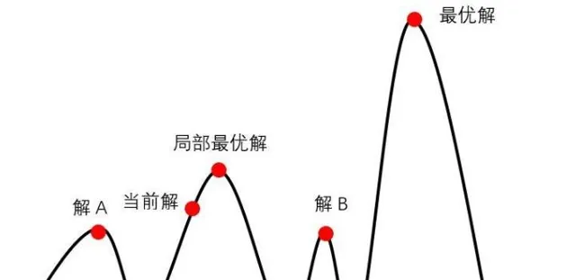
2、通过第1步得到最优位置可能还不是最优的位置,需要在最优位姿附近区域内采样 n 个位姿进行打分,分为四个方向和两个转向进行搜索,得分比较高的则为最优粒子位姿,使用的是爬山算法,之所以可以用爬山算法是因为在最优位姿附近进行小范围搜索采样的样本认为是符合高斯分布的,高斯分布为单峰函数,因此可以使用爬山算法。
3、 既然假设n 个位姿采样符合高斯分布,我们还需要求出期望 \mu 和方差 \sigma ,这就需要计算每个位姿的权重,并需要进行归一化,之后加权求和就可以得到期望,进而可以得到方差,也即最终我们得到的机器人最优位置服从:
x_{t}\sim N(\mu,\sigma^{2})
而权重的计算来自于激光雷达数据的似然得分:
 m_matcher
 .
 likelihoodAndScore
 (
 s
 ,
 l
 ,
 m_particles
 [
 i
 ].
 map
 ,
 m_particles
 [
 i
 ].
 pose
 ,
 plainReading
 );
权重计算公式:
 double
 f
 =
 (
 -
 1.
 /
 m_likelihoodSigma
 )
 *
 (
 bestMu
 *
 bestMu
 );
 //参数设置m_likelihoodSigma=0.075
累计权重就是粒子权重的累加。
6、 粒子权重归一化
归一化函数normalize()函数,其中还有对粒子差异性的判断,防止粒子耗散:
实现原理是:
假设有 n 个粒子,每个粒子的权重为 w^{i} ,其中权重最大值为 w_{max}
每个粒子经过公式换算后的权重:
w_{变换后}^{i}=e^{\frac{-1}{k*(w^{i}-w_{max})}}
所有粒子变换后的权重进行加和:
w_{所有}+=w_{变换后}^{i}
归一化:
w_{变换后}^{i}=\frac{w_{变换后}^{i}}{w_{所有}}
得到最终判断粒子是否发生的耗散的判据:
neff+=w_{变换后}^{i}
neff=\frac{1}{neff}
 //粒子差异化
 m_neff=0;
 for (std::vector<double>::iterator it=m_weights.begin(); it!=m_weights.end(); it++)
 {
 *it=*it/wcum;
 double w=*it;
 m_neff+=w*w;
 }
 m_neff=1./m_neff;
 //粒子权重归一化
 inline
 void
 GridSlamProcessor
 ::
 normalize
 ()
 {
 */
 /
 normalize
 *
 *
 the
 *
 *
 log
 *
 *
 m_weights
 *
 double
 gain
 =
 1.
 /
 (
 m_obsSigmaGain
 *
 m_particles
 .
 size
 ());
 double
 lmax
 =
 -
 std
 ::
 numeric_limits
 <
 double
 >::
 max
 ();
 for
 (
 ParticleVector
 ::
 iterator
 it
 =
 m_particles
 .
 begin
 ();
 it
 !=
 m_particles
 .
 end
 ();
 it
 ++
 )
 {
 lmax
 =
 it
 ->
 weight
 >
 lmax
 ?
 it
 ->
 weight
 :
 lmax
 ;
 }
 m_weights
 .
 clear
 ();
 double
 wcum
 =
 0
 ;
 m_neff
 =
 0
 ;
 for
 (
 std
 ::
 vector
 <
 Particle
 >::
 iterator
 it
 =
 m_particles
 .
 begin
 ();
 it
 !=
 m_particles
 .
 end
 ();
 it
 ++
 )
 {
 m_weights
 .
 push_back
 (
 exp
 (
 gain
 *
 (
 it
 ->
 weight
 -
 lmax
 )));
 wcum
 +=
 m_weights
 .
 back
 ();
 }
 //粒子差异化
 m_neff
 =
 0
 ;
 for
 (
 std
 ::
 vector
 <
 double
 >::
 iterator
 it
 =
 m_weights
 .
 begin
 ();
 it
 !=
 m_weights
 .
 end
 ();
 it
 ++
 )
 {
 *
 it
 =*
 it
 /
 wcum
 ;
 double
 w
 =*
 it
 ;
 m_neff
 +=
 w
 *
 w
 ;
 }
 m_neff
 =
 1.
 /
 m_neff
 ;
 }
主要代码实现:
 inline
 void
 GridSlamProcessor
 ::
 scanMatch
 (
 const
 double
 *
 plainReading
 ){
 double
 sumScore
 =
 0
 ;
 for
 (
 ParticleVector
 ::
 iterator
 it
 =
 m_particles
 .
 begin
 ();
 it
 !=
 m_particles
 .
 end
 ();
 it
 ++
 ){
 OrientedPoint
 corrected
 ;
 double
 score
 ,
 l
 ,
 s
 ;
 //第1步:得到最优匹配位置
 score
 =
 m_matcher
 .
 optimize
 (
 corrected
 ,
 it
 ->
 map
 ,
 it
 ->
 pose
 ,
 plainReading
 );
 if
 (
 score
 >
 m_minimumScore
 ){
 it
 ->
 pose
 =
 corrected
 ;
 }
 else
 {
 if
 (
 m_infoStream
 ){
 m_infoStream
 <<
 "Scan Matching Failed, using odometry. Likelihood="
 <<
 l
 <<
 std
 ::
 endl
 ;
 m_infoStream
 <<
 "lp:"
 <<
 m_lastPartPose
 .
 x
 <<
 " "
 <<
 m_lastPartPose
 .
 y
 <<
 " "
 <<
 m_lastPartPose
 .
 theta
 <<
 std
 ::
 endl
 ;
 m_infoStream
 <<
 "op:"
 <<
 m_odoPose
 .
 x
 <<
 " "
 <<
 m_odoPose
 .
 y
 <<
 " "
 <<
 m_odoPose
 .
 theta
 <<
 std
 ::
 endl
 ;
 }
 }
 //第2步:得到似然权重
 m_matcher
 .
 likelihoodAndScore
 (
 s
 ,
 l
 ,
 it
 ->
 map
 ,
 it
 ->
 pose
 ,
 plainReading
 );
 sumScore
 +=
 score
 ;
 it
 ->
 weight
 +=
 l
 ;
 it
 ->
 weightSum
 +=
 l
 ;
 m_matcher
 .
 invalidateActiveArea
 ();
 m_matcher
 .
 computeActiveArea
 (
 it
 ->
 map
 ,
 it
 ->
 pose
 ,
 plainReading
 );
 }
 double
 ScanMatcher
 ::
 optimize
 (
 OrientedPoint
 &
 pnew
 ,
 const
 ScanMatcherMap
 &
 map
 ,
 const
 OrientedPoint
 &
 init
 ,
 const
 double
 *
 readings
 )
 const
 {
 double
 bestScore
 =-
 1
 ;
 OrientedPoint
 currentPose
 =
 init
 ;
 double
 currentScore
 =
 score
 (
 map
 ,
 currentPose
 ,
 readings
 );
 double
 adelta
 =
 m_optAngularDelta
 ,
 ldelta
 =
 m_optLinearDelta
 ;
 unsigned
 int
 refinement
 =
 0
 ;
 enum
 Move
 {
 Front
 ,
 Back
 ,
 Left
 ,
 Right
 ,
 TurnLeft
 ,
 TurnRight
 ,
 Done
 };
 int
 c_iterations
 =
 0
 ;
 do
 {
 if
 (
 bestScore
 >=
 currentScore
 ){
 refinement
 ++
 ;
 adelta
 *=
 .5
 ;
 ldelta
 *=
 .5
 ;
 }
 bestScore
 =
 currentScore
 ;
 //		cout <<"score="<< currentScore << " refinement=" << refinement;
 //		cout << "pose=" << currentPose.x << " " << currentPose.y << " " << currentPose.theta << endl;
 OrientedPoint
 bestLocalPose
 =
 currentPose
 ;
 OrientedPoint
 localPose
 =
 currentPose
 ;
 Move
 move
 =
 Front
 ;
 do
 {
 localPose
 =
 currentPose
 ;
 switch
 (
 move
 ){
 case
 Front
 :
 localPose
 .
 x
 +=
 ldelta
 ;
 move
 =
 Back
 ;
 break
 ;
 case
 Back
 :
 localPose
 .
 x
 -=
 ldelta
 ;
 move
 =
 Left
 ;
 break
 ;
 case
 Left
 :
 localPose
 .
 y
 -=
 ldelta
 ;
 move
 =
 Right
 ;
 break
 ;
 case
 Right
 :
 localPose
 .
 y
 +=
 ldelta
 ;
 move
 =
 TurnLeft
 ;
 break
 ;
 case
 TurnLeft
 :
 localPose
 .
 theta
 +=
 adelta
 ;
 move
 =
 TurnRight
 ;
 break
 ;
 case
 TurnRight
 :
 localPose
 .
 theta
 -=
 adelta
 ;
 move
 =
 Done
 ;
 break
 ;
 default
 :
 ;
 }
 double
 localScore
 =
 score
 (
 map
 ,
 localPose
 ,
 readings
 );
 if
 (
 localScore
 >
 currentScore
 ){
 currentScore
 =
 localScore
 ;
 bestLocalPose
 =
 localPose
 ;
 }
 c_iterations
 ++
 ;
 }
 while
 (
 move
 !=
 Done
 );
 currentPose
 =
 bestLocalPose
 ;
 //cout << __func__ << "currentScore=" << currentScore<< endl;
 //here we look for the best move;
 }
 while
 (
 currentScore
 >
 bestScore
 ||
 refinement
 <
 m_optRecursiveIterations
 );
 //cout << __func__ << "bestScore=" << bestScore<< endl;
 //cout << __func__ << "iterations=" << c_iterations<< endl;
 pnew
 =
 currentPose
 ;
 return
 bestScore
 ;
 }
7、 粒子重采样,增加多样性,增加机器人位姿预测范围
重采样函数resample()
重采样算法采用转盘赌算法,当然这个算法是有一些缺陷的,感兴趣的可以查看更多的重采样方法。

算法实现的基本思想:
比如有15个粒子,经过迭代后,发现有5个粒子权重已经很低了,也就是已经退化了,因此我们需要将其剔除,从剩下的10个中再抽样5个,保持整体15个粒子不变。
首先求得这10个粒子权重的均值:
interval=\frac{1}{n}\sum_{1}^{10}{w_{t}^{i}}(i=1,2,...10)
随机抽样一个初始值:
target=interval*rand(Numer)比如target=interval*10
接着按照如下伪代码进行采样:
for\ \ m=1\ to\ \ 10\ \ do\\target=interval*rand(Numer)\\i=1\\while\ \ target>interval\\i=i+1\\interval+=interval\\end\ \ while\\add \ \ \ x^{i}\\end for\\ 代码实现:
 std
 ::
 vector
 <
 Particle
 >
 uniform_resampler
 <
 Particle
 ,
 Numeric
 >::
 resample
 (
 const
 typename
 std
 ::
 vector
 <
 Particle
 >&
 particles
 ,
 int
 nparticles
 )
 const
 {
 Numeric
 cweight
 =
 0
 ;
 //compute the cumulative weights
 unsigned
 int
 n
 =
 0
 ;
 for
 (
 typename
 std
 ::
 vector
 <
 Particle
 >::
 const_iterator
 it
 =
 particles
 .
 begin
 ();
 it
 !=
 particles
 .
 end
 ();
 ++
 it
 ){
 cweight
 +=
 (
 Numeric
 )
 *
 it
 ;
 n
 ++
 ;
 }
 if
 (
 nparticles
 >
 0
 )
 n
 =
 nparticles
 ;
 //weight of the particles after resampling
 double
 uw
 =
 1.
 /
 n
 ;
 //compute the interval
 Numeric
 interval
 =
 cweight
 /
 n
 ;
 //compute the initial target weight
 Numeric
 target
 =
 interval
 *::
 drand48
 ();
 //compute the resampled indexes
 cweight
 =
 0
 ;
 std
 ::
 vector
 <
 Particle
 >
 resampled
 ;
 n
 =
 0
 ;
 unsigned
 int
 i
 =
 0
 ;
 for
 (
 typename
 std
 ::
 vector
 <
 Particle
 >::
 const_iterator
 it
 =
 particles
 .
 begin
 ();
 it
 !=
 particles
 .
 end
 ();
 ++
 it
 ,
 ++
 i
 ){
 cweight
 +=
 (
 Numeric
 )
 *
 it
 ;
 while
 (
 cweight
 >
 target
 ){
 resampled
 .
 push_back
 (
 *
 it
 );
 resampled
 .
 back
 ().
 setWeight
 (
 uw
 );
 target
 +=
 interval
 ;
 }
 }
 return
 resampled
 ;
 }
8、粒子数据结构形式
整个代码中粒子的数据结构可谓是最重要的。
节点,由于每个粒子都存储着历史的轨迹和地图,因此需要一个树结构来存储这些数据,树结构是以节点node的形式组织起来的,一个节点包括父节点和子节点,这样整个节点就可以彼此找到。
 TNode
 (
 const
 OrientedPoint
 &
 pose
 ,
 double
 weight
 ,
 TNode
 *
 parent
 =
 0
 ,
 unsigned
 int
 childs
 =
 0
 );
 /**Destroys a tree node, and consistently updates the tree. If a node whose parent has only one child is deleted,
 also the parent node is deleted. This because the parent will not be reacheable anymore in the trajectory tree.*/
 ~
 TNode
 ();
 /**The pose of the robot*/
 //机器人位姿
 OrientedPoint
 pose
 ;
 //父节点
 TNode
 *
 parent
 ;
 /**The range reading to which this node is associated*/
 //激光雷达数据
 const
 RangeReading
 *
 reading
 ;
 };
粒子数据结构:
 struct
 Particle
 {
 Particle
 (
 const
 ScanMatcherMap
 &
 map
 );
 /** @returns the weight of a particle */
 inline
 operator
 double
 ()
 const
 {
 return
 weight
 ;}
 /** @returns the pose of a particle */
 inline
 operator
 OrientedPoint
 ()
 const
 {
 return
 pose
 ;}
 /** sets the weight of a particle
 @param w the weight
 */
 inline
 void
 setWeight
 (
 double
 w
 )
 {
 weight
 =
 w
 ;}
 /** The map */
 ScanMatcherMap
 map
 ;
 /** The pose of the robot */
 OrientedPoint
 pose
 ;
 /** The pose of the robot at the previous time frame (used for computing thr odometry displacements) */
 OrientedPoint
 previousPose
 ;
 /** The weight of the particle */
 double
 weight
 ;
 /** The cumulative weight of the particle */
 double
 weightSum
 ;
 double
 gweight
 ;
 /** The index of the previous particle in the trajectory tree */
 int
 previousIndex
 ;
 /** Entry to the trajectory tree */
 TNode
 *
 node
 ;
 };
六、地图更新
用到的函数为:updateMap()
知乎作者的一篇文章,说明了占据地图是如何创建的,这里就不再介绍了。
小白学移动机器人:占据栅格地图构建(Occupancy Grid Map)
 SlamGMapping
 ::
 updateMap
 (
 const
 sensor_msgs
 ::
 LaserScan
 &
 scan
 )
 {
 ROS_DEBUG
 (
 "Update map"
 );
 boost
 ::
 mutex
 ::
 scoped_lock
 map_lock
 (
 map_mutex_
 );
 GMapping
 ::
 ScanMatcher
 matcher
 ;
 matcher
 .
 setLaserParameters
 (
 scan
 .
 ranges
 .
 size
 (),
 &
 (
 laser_angles_
 [
 0
 ]),
 gsp_laser_
 ->
 getPose
 ());
 matcher
 .
 setlaserMaxRange
 (
 maxRange_
 );
 matcher
 .
 setusableRange
 (
 maxUrange_
 );
 matcher
 .
 setgenerateMap
 (
 true
 );
 GMapping
 ::
 GridSlamProcessor
 ::
 Particle
 best
 =
 gsp_
 ->
 getParticles
 ()[
 gsp_
 ->
 getBestParticleIndex
 ()];
 std_msgs
 ::
 Float64
 entropy
 ;
 entropy
 .
 data
 =
 computePoseEntropy
 ();
 if
 (
 entropy
 .
 data
 >
 0.0
 )
 entropy_publisher_
 .
 publish
 (
 entropy
 );
 if
 (
 !
 got_map_
 )
 {
 map_
 .
 map
 .
 info
 .
 resolution
 =
 delta_
 ;
 map_
 .
 map
 .
 info
 .
 origin
 .
 position
 .
 x
 =
 0.0
 ;
 map_
 .
 map
 .
 info
 .
 origin
 .
 position
 .
 y
 =
 0.0
 ;
 map_
 .
 map
 .
 info
 .
 origin
 .
 position
 .
 z
 =
 0.0
 ;
 map_
 .
 map
 .
 info
 .
 origin
 .
 orientation
 .
 x
 =
 0.0
 ;
 map_
 .
 map
 .
 info
 .
 origin
 .
 orientation
 .
 y
 =
 0.0
 ;
 map_
 .
 map
 .
 info
 .
 origin
 .
 orientation
 .
 z
 =
 0.0
 ;
 map_
 .
 map
 .
 info
 .
 origin
 .
 orientation
 .
 w
 =
 1.0
 ;
 }
 GMapping
 ::
 Point
 center
 ;
 center
 .
 x
 =
 (
 xmin_
 +
 xmax_
 )
 /
 2.0
 ;
 center
 .
 y
 =
 (
 ymin_
 +
 ymax_
 )
 /
 2.0
 ;
 GMapping
 ::
 ScanMatcherMap
 smap
 (
 center
 ,
 xmin_
 ,
 ymin_
 ,
 xmax_
 ,
 ymax_
 ,
 delta_
 );
 ROS_DEBUG
 (
 "Trajectory tree:"
 );
 for
 (
 GMapping
 ::
 GridSlamProcessor
 ::
 TNode
 *
 n
 =
 best
 .
 node
 ;
 n
 ;
 n
 =
 n
 ->
 parent
 )
 {
 ROS_DEBUG
 (
 " %.3f %.3f %.3f"
 ,
 n
 ->
 pose
 .
 x
 ,
 n
 ->
 pose
 .
 y
 ,
 n
 ->
 pose
 .
 theta
 );
 if
 (
 !
 n
 ->
 reading
 )
 {
 ROS_DEBUG
 (
 "Reading is NULL"
 );
 continue
 ;
 }
 matcher
 .
 invalidateActiveArea
 ();
 matcher
 .
 computeActiveArea
 (
 smap
 ,
 n
 ->
 pose
 ,
 &
 ((
 *
 n
 ->
 reading
 )[
 0
 ]));
 matcher
 .
 registerScan
 (
 smap
 ,
 n
 ->
 pose
 ,
 &
 ((
 *
 n
 ->
 reading
 )[
 0
 ]));
 }
 // the map may have expanded, so resize ros message as well
 if
 (
 map_
 .
 map
 .
 info
 .
 width
 !=
 (
 unsigned
 int
 )
 smap
 .
 getMapSizeX
 ()
 ||
 map_
 .
 map
 .
 info
 .
 height
 !=
 (
 unsigned
 int
 )
 smap
 .
 getMapSizeY
 ())
 {
 // NOTE: The results of ScanMatcherMap::getSize() are different from the parameters given to the constructor
 // so we must obtain the bounding box in a different way
 GMapping
 ::
 Point
 wmin
 =
 smap
 .
 map2world
 (
 GMapping
 ::
 IntPoint
 (
 0
 ,
 0
 ));
 GMapping
 ::
 Point
 wmax
 =
 smap
 .
 map2world
 (
 GMapping
 ::
 IntPoint
 (
 smap
 .
 getMapSizeX
 (),
 smap
 .
 getMapSizeY
 ()));
 xmin_
 =
 wmin
 .
 x
 ;
 ymin_
 =
 wmin
 .
 y
 ;
 xmax_
 =
 wmax
 .
 x
 ;
 ymax_
 =
 wmax
 .
 y
 ;
 ROS_DEBUG
 (
 "map size is now %dx%d pixels (%f,%f)-(%f, %f)"
 ,
 smap
 .
 getMapSizeX
 (),
 smap
 .
 getMapSizeY
 (),
 xmin_
 ,
 ymin_
 ,
 xmax_
 ,
 ymax_
 );
 map_
 .
 map
 .
 info
 .
 width
 =
 smap
 .
 getMapSizeX
 ();
 map_
 .
 map
 .
 info
 .
 height
 =
 smap
 .
 getMapSizeY
 ();
 map_
 .
 map
 .
 info
 .
 origin
 .
 position
 .
 x
 =
 xmin_
 ;
 map_
 .
 map
 .
 info
 .
 origin
 .
 position
 .
 y
 =
 ymin_
 ;
 map_
 .
 map
 .
 data
 .
 resize
 (
 map_
 .
 map
 .
 info
 .
 width
 *
 map_
 .
 map
 .
 info
 .
 height
 );
 ROS_DEBUG
 (
 "map origin: (%f, %f)"
 ,
 map_
 .
 map
 .
 info
 .
 origin
 .
 position
 .
 x
 ,
 map_
 .
 map
 .
 info
 .
 origin
 .
 position
 .
 y
 );
 }
 for
 (
 int
 x
 =
 0
 ;
 x
 <
 smap
 .
 getMapSizeX
 ();
 x
 ++
 )
 {
 for
 (
 int
 y
 =
 0
 ;
 y
 <
 smap
 .
 getMapSizeY
 ();
 y
 ++
 )
 {
 /// @todo Sort out the unknown vs. free vs. obstacle thresholding
 GMapping
 ::
 IntPoint
 p
 (
 x
 ,
 y
 );
 double
 occ
 =
 smap
 .
 cell
 (
 p
 );
 assert
 (
 occ
 <=
 1.0
 );
 if
 (
 occ
 <
 0
 )
 map_
 .
 map
 .
 data
 [
 MAP_IDX
 (
 map_
 .
 map
 .
 info
 .
 width
 ,
 x
 ,
 y
 )]
 =
 -
 1
 ;
 else
 if
 (
 occ
 >
 occ_thresh_
 )
 {
 //map_.map.data[MAP_IDX(map_.map.info.width, x, y)] = (int)round(occ*100.0);
 map_
 .
 map
 .
 data
 [
 MAP_IDX
 (
 map_
 .
 map
 .
 info
 .
 width
 ,
 x
 ,
 y
 )]
 =
 100
 ;
 }
 else
 map_
 .
 map
 .
 data
 [
 MAP_IDX
 (
 map_
 .
 map
 .
 info
 .
 width
 ,
 x
 ,
 y
 )]
 =
 0
 ;
 }
 }
 got_map_
 =
 true
 ;
 //make sure to set the header information on the map
 map_
 .
 map
 .
 header
 .
 stamp
 =
 ros
 ::
 Time
 ::
 now
 ();
 map_
 .
 map
 .
 header
 .
 frame_id
 =
 tf_
 .
 resolve
 (
 map_frame_
 );
 sst_
 .
 publish
 (
 map_
 .
 map
 );
 sstm_
 .
 publish
 (
 map_
 .
 map
 .
 info
 );
 }
七、结束语
最后,GMapping不是万能的,它只是在特定历史时期提出的当时最好的方案。比如Gmapping参考了里程计的数据,可以使建图更精确,相比于Hector SLAM,GMapping对激光雷达频率要求低、鲁棒性更高。
但一旦里程计打滑,GMapping地图创建就会出现问题,一般会结合多传感器和障碍物点云匹配来进行矫正。
如今,一提到SLAM建图,都少不了谷歌的Cartographer,在实用性方面其霸主地位迄今也无法撼动。
但GMapping作为特定时代的产物,依然有许多值得借鉴的东西,程序简洁的架构和思想,依然非常值得我们学习,注定在SLAM的历史上留下浓墨重彩的一笔。


